Group Models

Here you will learn how to combine models together into a larger, more complete, model of a given system. This is a powerful and necessary capability when analysing objects in crowded environments. As telescopes achieve ever deeper photometry we have learned that all environments are crowded when projected onto the sky!

import astrophot as ap
import numpy as np
import torch
from astropy.io import fits
import matplotlib.pyplot as plt
from scipy.stats import iqr

# first let's download an image to play with
hdu = fits.open("https://www.legacysurvey.org/viewer/fits-cutout?ra=4.5934&dec=30.0702&size=750&layer=ls-dr9&pixscale=0.262&bands=r")
target_data = np.array(hdu[0].data, dtype = np.float64)

target1 = ap.image.Target_Image(
    data = target_data,
    pixelscale = 0.262,
    zeropoint = 22.5,
)

fig1, ax1 = plt.subplots(figsize = (8,8))
ap.plots.target_image(fig1, ax1, target1)
plt.show()

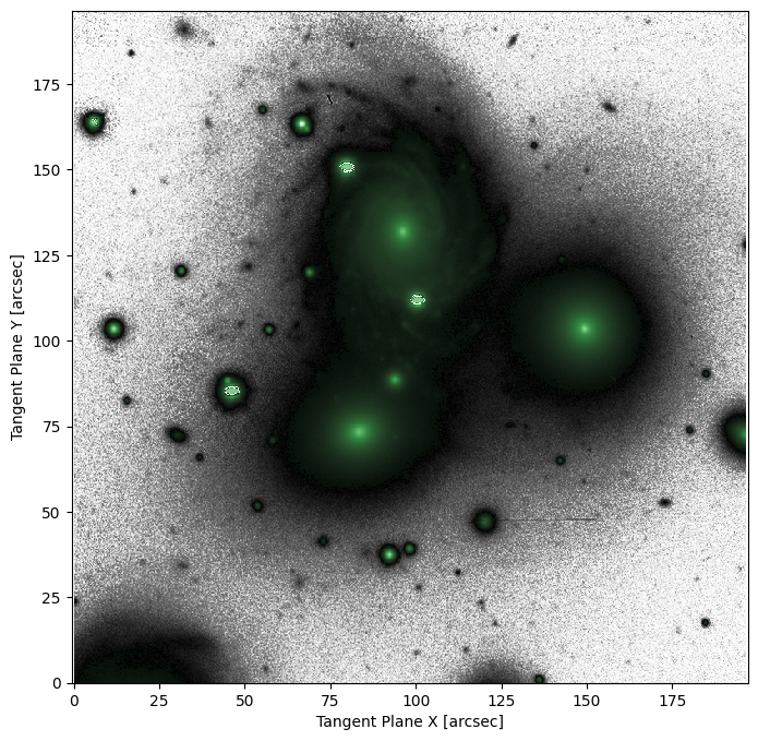
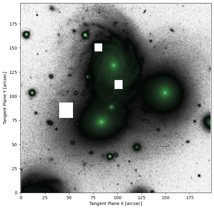
# We can see that there are some blown out stars in the image. There isn't much that can be done with them except
# to mask them. A very careful modeller would only mask the blown out pixels and then try to fit the rest, but
# today we are not very careful modellers.
mask = np.zeros(target_data.shape, dtype = bool)
mask[410:445,371:402] = True
mask[296:357 ,151:206] = True
mask[558:590,291:322] = True
# Note that it is also possible to set a mask just for an individual model. Simply create a mask in the same way as
# above. Just note that the mask should have the same shape as the model window instead of the whole image.

pixelscale = 0.262
target2 = ap.image.Target_Image(
    data = target_data,
    pixelscale = pixelscale,
    zeropoint = 22.5,
    mask = mask, # now the target image has a mask of bad pixels
    variance = 0.001*np.abs(target_data + iqr(target_data,rng=[16,84])/2), # we create a variance image, if the image is in counts then variance image = image, in this case the sky has been subtracted so we add back in a certain amount of variance
)

fig2, ax2 = plt.subplots(figsize = (8,8))
ap.plots.target_image(fig2, ax2, target2)
plt.show()

Group Model

A group model takes a list of other AstroPhot_Model objects and tracks them such that they can be treated as a single larger model. When “initialize” is called on the group model, it simply calls “initialize” on all the individual models. The same is true for a number of other functions like finalize, sample, and so on. For fitting, however, the group model will collect the parameters from all the models together and pass them along as one group to the optimizer. When saving a group model, all the model states will be collected together into one large file.

The main difference when constructing a group model is that you must first create all the sub models that will go in it. Once constructed, a group model behaves just like any other model, in fact they are all built from the same base class.

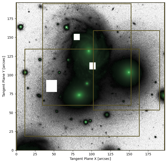
# first we make the list of models to fit

# Note that we do not assign a target to these models at construction. This is just a choice of style, it is possible
# to provide the target to each model separately if you wish. Note as well that since a target isn't provided we need
# to give the windows in arcsec instead of pixels, to do this we provide the window in the format (xmin,xmax,ymin,ymax)
model_kwargs = [
    {"name": "sky", "model_type": "flat sky model", "window": [[0,750],[0,750]]},
    {"name": "NGC0070", "model_type": "spline galaxy model", "window": [[133,581],[229,744]]},
    {"name": "NGC0071", "model_type": "spline galaxy model", "window": [[43,622],[72,513]]},
    {"name": "NGC0068", "model_type": "spline galaxy model", "window": [[390,726],[204,607]]},
]

model_list = []
for M in model_kwargs:
    model_list.append(ap.models.AstroPhot_Model(target = target2, **M))

VV166Group = ap.models.AstroPhot_Model(name = "VV166 Group", model_type = "group model", models = model_list, target = target2)

fig3, ax3 = plt.subplots(figsize = (8,8))
ap.plots.target_image(fig3, ax3, VV166Group.target)
ap.plots.model_window(fig3, ax3, VV166Group)
plt.show()

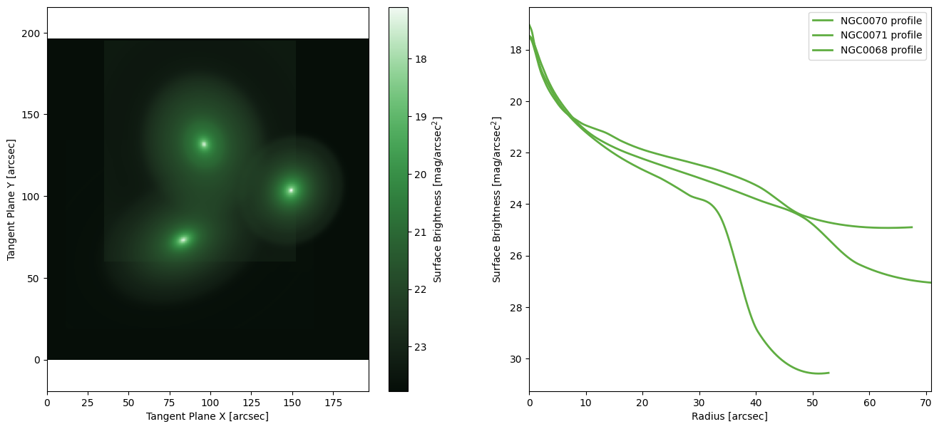
# See if AstroPhot can figure out starting parameters for these galaxies
VV166Group.initialize()

# The results are reasonable starting points, though far from a good model
fig4, ax4 = plt.subplots(1,2,figsize = (16,7))
ap.plots.model_image(fig4, ax4[0], VV166Group)
for M in VV166Group.models.values():
    if M.name == "sky": continue
    ap.plots.radial_light_profile(fig4, ax4[1], M)
plt.legend()
plt.show()

# Allow AstroPhot to fit the target image with all 3 models simultaneously. In total this is about 80 parameters!
result = ap.fit.LM(VV166Group, verbose = 1).fit()
print(result.message)

Chi^2/DoF: 8.512829252335521, L: 1.0
Chi^2/DoF: 8.376172677180785, L: 1.6666666666666667
Chi^2/DoF: 7.7431411993199255, L: 0.5555555555555556
Chi^2/DoF: 7.579383923177304, L: 0.9259259259259259
Chi^2/DoF: 7.076326370057542, L: 0.30864197530864196
Chi^2/DoF: 6.955055298306867, L: 0.51440329218107
Chi^2/DoF: 6.748758023878665, L: 0.17146776406035666
Chi^2/DoF: 6.663235907050428, L: 0.05715592135345222
Chi^2/DoF: 6.633867406844346, L: 0.09525986892242037
Chi^2/DoF: 6.6032026041723455, L: 0.031753289640806794
Chi^2/DoF: 6.602689789003671, L: 0.010584429880268932
Chi^2/DoF: 6.60266230587986, L: 0.44101791167787224
Chi^2/DoF: 6.602658681708982, L: 0.7350298527964537
Chi^2/DoF: 6.602658068286201, L: 1.2250497546607562
Chi^2/DoF: 6.602657938151657, L: 2.04174959110126
Chi^2/DoF: 6.602657620928402, L: 0.6805831970337534
Chi^2/DoF: 6.602657620927289, L: 708.940830243493
Chi^2/DoF: 6.602657620926983, L: 1181.5680504058216
Chi^2/DoF: 6.6026576209252275, L: 393.85601680194054
Final Chi^2/DoF: 6.602657620923972, L: 1969.2800840097027. Converged: success by immobility. Convergence not guaranteed
success by immobility. Convergence not guaranteed

# Now we can see what the fitting has produced
fig5, ax5 = plt.subplots(1,3,figsize = (17,5))
ap.plots.model_image(fig5, ax5[0], VV166Group)
for M in VV166Group.models.values():
    if M.name == "sky": continue
    ap.plots.radial_light_profile(fig5, ax5[1], M)
    ap.plots.radial_median_profile(fig5, ax5[1], M)
ax5[1].legend()
ap.plots.residual_image(fig5, ax5[2], VV166Group)
plt.show()

# we can also see that the data profiles which just take a median for all pixels at a given radius are no longer
# helpful when we have overlapping systems. The medians are biased high by the neighboring galaxies

# To access parameters in a group model you use the same syntax as usual, but with the model name as well:
print(VV166Group["NGC0070:PA"])
print(VV166Group["NGC0071:PA"])

PA: 0.15524958801725042 +- 0.06 [radians], limits: (0.0, 3.141592653589793), cyclic
PA: 1.8680043543430165 +- 0.06 [radians], limits: (0.0, 3.141592653589793), cyclic

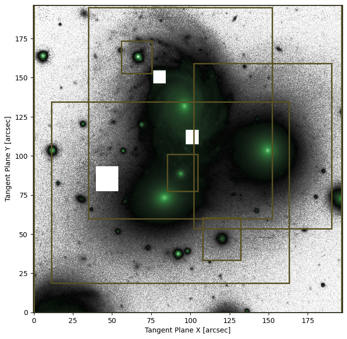
# The model will improve the more galaxies in the system we include
# By adding models now, we keep the fitted parameters from before.
VV166Group.add_model(ap.models.AstroPhot_Model(name = "litte 1", model_type = "sersic galaxy model", target = target2, window = [[325,400],[295,386]]))
VV166Group.add_model(ap.models.AstroPhot_Model(name = "litte 2", model_type = "sersic galaxy model", target = target2, window = [[412,504],[127,231]]))
VV166Group.add_model(ap.models.AstroPhot_Model(name = "litte 3", model_type = "sersic galaxy model", target = target2, window = [[214,288],[583,662]]))

fig6, ax6 = plt.subplots(figsize = (8,8))
ap.plots.target_image(fig6, ax6, VV166Group.target)
ap.plots.model_window(fig6, ax6, VV166Group)
plt.show()

# Initialize will only set parameter values for the new models, the old ones will just be skipped
VV166Group.initialize()

result = ap.fit.LM(VV166Group, verbose = 1).fit()
print(result.message)

Chi^2/DoF: 5.253002956525187, L: 1.0
Chi^2/DoF: 5.0038949960035275, L: 1.6666666666666667
Chi^2/DoF: 4.969093493217347, L: 0.5555555555555556
Chi^2/DoF: 4.879343923691995, L: 0.0205761316872428
Chi^2/DoF: 4.852323279250886, L: 0.03429355281207133
Chi^2/DoF: 4.848173065848449, L: 0.05715592135345222
Chi^2/DoF: 4.846858913259821, L: 0.09525986892242037
Chi^2/DoF: 4.845709613389932, L: 0.031753289640806794
Chi^2/DoF: 4.845562350434843, L: 0.26461074700672327
Chi^2/DoF: 4.844974340180937, L: 0.08820358233557442
Chi^2/DoF: 4.843891751247251, L: 0.14700597055929068
Chi^2/DoF: 4.843878704279775, L: 1.2250497546607557
Chi^2/DoF: 4.843120776556546, L: 0.4083499182202519
Chi^2/DoF: 4.842730281054922, L: 0.6805831970337533
Chi^2/DoF: 4.842639881302593, L: 1.1343053283895888
Chi^2/DoF: 4.842625821615503, L: 1.8905088806493147
Chi^2/DoF: 4.841498068851339, L: 0.6301696268831048
Chi^2/DoF: 4.841040701952689, L: 1.0502827114718414
Chi^2/DoF: 4.840950406828487, L: 1.7504711857864024
Chi^2/DoF: 4.806997264827536, L: 0.5834903952621341
Chi^2/DoF: 4.795780551612838, L: 0.19449679842071135
Chi^2/DoF: 4.788255230790208, L: 0.00026679944913677824
Chi^2/DoF: 4.7871249056327425, L: 3.659800399681458e-07
Chi^2/DoF: 4.786986082915262, L: 4.51827209837217e-09
Chi^2/DoF: 4.786974597420668, L: 1.50609069945739e-09
Final Chi^2/DoF: 4.7869651381749065, L: 1.50609069945739e-09. Converged: success
success

# Now we can see what the fitting has produced
fig7, ax7 = plt.subplots(1,3,figsize = (17,5))
ap.plots.model_image(fig7, ax7[0], VV166Group)
# let's just plot the 3 main object profiles
for M in VV166Group.models.values():
    if not "NGC" in M.name: continue
    ap.plots.radial_light_profile(fig7, ax7[1], M)
ax7[1].legend()
ax7[1].set_ylim([27,15])
ap.plots.residual_image(fig7, ax7[2], VV166Group)
plt.show()

Which is even better than before. As more models are added, the fit should improve. In principle one could model eventually add models for every little smudge in the image. In practice, it is often better to just mask anything below a certain size.

Working with segmentation maps

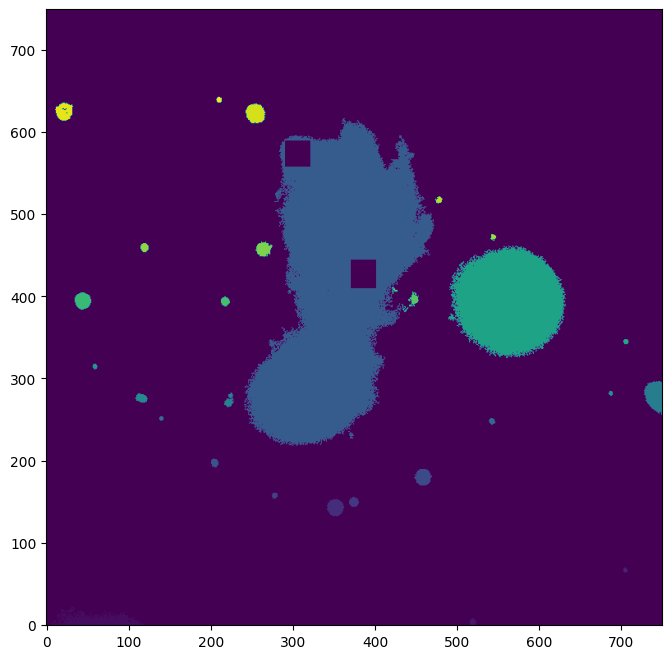
A segmentation map provides information about the contents of an image. It gives the location and shape of any object which the algorithm was able to separate out and identify. This is exactly the information needed to construct the windows for a collection of AstroPhot models.

Photutils provides an easy to use segmentation map implimentation so we use it here for simplicity. In many cases it may be required to use a more detailed segmentation map algorithm such as those implimented in Source Extractor and ProFound (among others), the principle is the same however since the end product for all of them has the same format.

#########################################
# NOTE: photutils is not a dependency of AstroPhot, make sure you run: pip install photutils
# if you dont already have that package. Also note that you can use any segmentation map
# code, we just use photutils here because it is very easy.
#########################################
from photutils.segmentation import detect_sources
segmap = detect_sources(target_data, threshold = 0.1, npixels = 20, mask = mask) # threshold and npixels determined just by playing around with the values
fig8, ax8 = plt.subplots(figsize=(8,8))
ax8.imshow(segmap, origin = "lower")
plt.show()

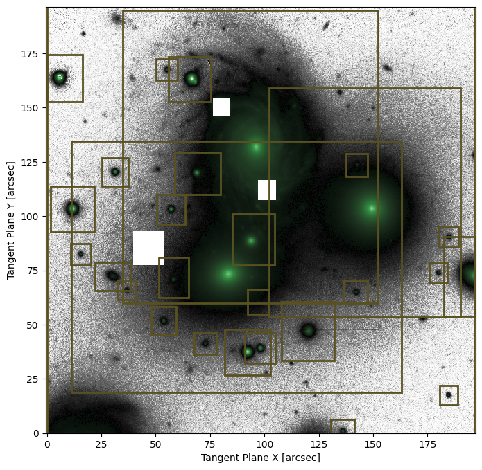
# This will convert the segmentation map into boxes that enclose the identified pixels
windows = ap.utils.initialize.windows_from_segmentation_map(segmap.data)
# Next we filter out any segments which are too big, these are the NGC models we already have set up
windows = ap.utils.initialize.filter_windows(windows, max_size = 100)
# Next we scale up the windows so that AstroPhot can fit the faint parts of each object as well
windows = ap.utils.initialize.scale_windows(windows, image_shape = target_data.shape, expand_scale = 3, expand_border = 10)

del windows[20] # this is a segmented chunk of spiral arm, not a galaxy
del windows[23] # this is a segmented chunk of spiral arm, not a galaxy
del windows[24] # this is a segmented chunk of spiral arm, not a galaxy
del windows[28] # this is a segmented chunk of spiral arm, not a galaxy
del windows[29] # this is a repeat of little 2
del windows[7] # this is a repeat of little 3
print(windows)

{2: [[499, 540], [0, 24]], 3: [[689, 721], [49, 84]], 4: [[312, 392], [102, 182]], 5: [[348, 401], [123, 176]], 6: [[259, 297], [138, 176]], 8: [[183, 227], [172, 222]], 10: [[352, 390], [209, 253]], 11: [[522, 563], [227, 268]], 12: [[124, 156], [235, 267]], 13: [[697, 750], [206, 346]], 14: [[196, 249], [238, 309]], 15: [[85, 147], [251, 301]], 16: [[671, 703], [264, 299]], 17: [[42, 77], [295, 333]], 19: [[688, 723], [327, 362]], 21: [[6, 83], [354, 434]], 22: [[193, 243], [367, 420]], 25: [[225, 305], [420, 494]], 26: [[96, 143], [434, 484]], 27: [[525, 563], [451, 492]], 30: [[0, 63], [583, 666]], 31: [[191, 229], [620, 658]]}

# Now we use all the windows to add to the list of models
seg_models = []
for win in windows:
    seg_models.append({"name": f"minor object {win:02d}", "window": windows[win], "model_type": "sersic galaxy model", "target": target2})

# we make a new set of models for simplicity
for M in seg_models:
    VV166Group.add_model(ap.models.AstroPhot_Model(**M))

VV166Group.initialize()

fig9, ax9 = plt.subplots(figsize = (8,8))
ap.plots.target_image(fig9, ax9, VV166Group.target)
ap.plots.model_window(fig9, ax9, VV166Group)
plt.show()

# This is now a very complex model composed of about 30 sub-models! In total 253 parameters! While it is
# possible for the AstroPhot Levenberg-Marquardt (LM) algorithm to fully optimize this model, it is faster in this
# case to apply an iterative fit. AstroPhot will apply LM optimization one model at a time and cycle through all
# the models until the results converge. See the tutorial on AstroPhot fitting for more details on the fit methods.
result = ap.fit.Iter(VV166Group, verbose = 1, method_kwargs = {"max_iter": 5}).fit()
print(result.message)

# Other technqiues that can help for difficult fits:
# - Try running some gradient descent steps (maybe 100) before doing LM
# - Try changing the initial parameters. AstroPhot seeks a local minimum so make sure its the right one!
# - Fit the large models in the frame first, then add in the smaller ones (thats what we've done in this tutorial)
# - Fit a simplier model (say a sersic or exponential instead of spline) first, then use that to initialize the complex model
# - Mix and match optimizers, if one gets stuck another may be better suited for that area of parameter space

--------iter-------
sky
NGC0070
NGC0071
NGC0068
litte 1
litte 2
litte 3
minor object 02
minor object 03
minor object 04
minor object 05
minor object 06
minor object 08
minor object 10
minor object 11
minor object 12
minor object 13
minor object 14
minor object 15
minor object 16
minor object 17
minor object 19
minor object 21
minor object 22
minor object 25
minor object 26
minor object 27
minor object 30
minor object 31
Update Chi^2 with new parameters
Loss: 2.349551540624039
--------iter-------
sky
NGC0070
NGC0071
NGC0068
litte 1
litte 2
litte 3
minor object 02
minor object 03
minor object 04
minor object 05
minor object 06
minor object 08
minor object 10
minor object 11
minor object 12
minor object 13
minor object 14
minor object 15
minor object 16
minor object 17
minor object 19
minor object 21
minor object 22
minor object 25
minor object 26
minor object 27
minor object 30
minor object 31
Update Chi^2 with new parameters
Loss: 2.289814484237822
--------iter-------
sky
NGC0070
NGC0071
NGC0068
litte 1
litte 2
litte 3
minor object 02
minor object 03
minor object 04
minor object 05
minor object 06
minor object 08
minor object 10
minor object 11
minor object 12
minor object 13
minor object 14
minor object 15
minor object 16
minor object 17
minor object 19
minor object 21
minor object 22
minor object 25
minor object 26
minor object 27
minor object 30
minor object 31
Update Chi^2 with new parameters
Loss: 2.2307467052693397
--------iter-------
sky
NGC0070
NGC0071
NGC0068
litte 1
litte 2
litte 3
minor object 02
minor object 03
minor object 04
minor object 05
minor object 06
minor object 08
minor object 10
minor object 11
minor object 12
minor object 13
minor object 14
minor object 15
minor object 16
minor object 17
minor object 19
minor object 21
minor object 22
minor object 25
minor object 26
minor object 27
minor object 30
minor object 31
Update Chi^2 with new parameters
Loss: 2.1254155864729958
--------iter-------
sky
NGC0070
NGC0071
NGC0068
litte 1
litte 2
litte 3
minor object 02
minor object 03
minor object 04
minor object 05
minor object 06
minor object 08
minor object 10
minor object 11
minor object 12
minor object 13
minor object 14
minor object 15
minor object 16
minor object 17
minor object 19
minor object 21
minor object 22
minor object 25
minor object 26
minor object 27
minor object 30
minor object 31
Update Chi^2 with new parameters
Loss: 2.1065758023848566
--------iter-------
sky
NGC0070
NGC0071
NGC0068
litte 1
litte 2
litte 3
minor object 02
minor object 03
minor object 04
minor object 05
minor object 06
minor object 08
minor object 10
minor object 11
minor object 12
minor object 13
minor object 14
minor object 15
minor object 16
minor object 17
minor object 19
minor object 21
minor object 22
minor object 25
minor object 26
minor object 27
minor object 30
minor object 31
Update Chi^2 with new parameters
Loss: 2.093203650899399
--------iter-------
sky
NGC0070
NGC0071
NGC0068
litte 1
litte 2
litte 3
minor object 02
minor object 03
minor object 04
minor object 05
minor object 06
minor object 08
minor object 10
minor object 11
minor object 12
minor object 13
minor object 14
minor object 15
minor object 16
minor object 17
minor object 19
minor object 21
minor object 22
minor object 25
minor object 26
minor object 27
minor object 30
minor object 31
Update Chi^2 with new parameters
Loss: 2.035271465603128
--------iter-------
sky
NGC0070
NGC0071
NGC0068
litte 1
litte 2
litte 3
minor object 02
minor object 03
minor object 04
minor object 05
minor object 06
minor object 08
minor object 10
minor object 11
minor object 12
minor object 13
minor object 14
minor object 15
minor object 16
minor object 17
minor object 19
minor object 21
minor object 22
minor object 25
minor object 26
minor object 27
minor object 30
minor object 31
Update Chi^2 with new parameters
Loss: 2.028520580295159
--------iter-------
sky
NGC0070
NGC0071
NGC0068
litte 1
litte 2
litte 3
minor object 02
minor object 03
minor object 04
minor object 05
minor object 06
minor object 08
minor object 10
minor object 11
minor object 12
minor object 13
minor object 14
minor object 15
minor object 16
minor object 17
minor object 19
minor object 21
minor object 22
minor object 25
minor object 26
minor object 27
minor object 30
minor object 31
Update Chi^2 with new parameters
Loss: 2.0283736660559204
--------iter-------
sky
NGC0070
NGC0071
NGC0068
litte 1
litte 2
litte 3
minor object 02
minor object 03
minor object 04
minor object 05
minor object 06
minor object 08
minor object 10
minor object 11
minor object 12
minor object 13
minor object 14
minor object 15
minor object 16
minor object 17
minor object 19
minor object 21
minor object 22
minor object 25
minor object 26
minor object 27
minor object 30
minor object 31
Update Chi^2 with new parameters
Loss: 2.0283531232933636
success

# Indeed the fit converges successfully! These tricks are really useful for complex fits.

# Now we can see what the fitting has produced
fig10, ax10 = plt.subplots(1,2,figsize = (16,7))
ap.plots.model_image(fig10, ax10[0], VV166Group)
ap.plots.residual_image(fig10, ax10[1], VV166Group)
plt.show()

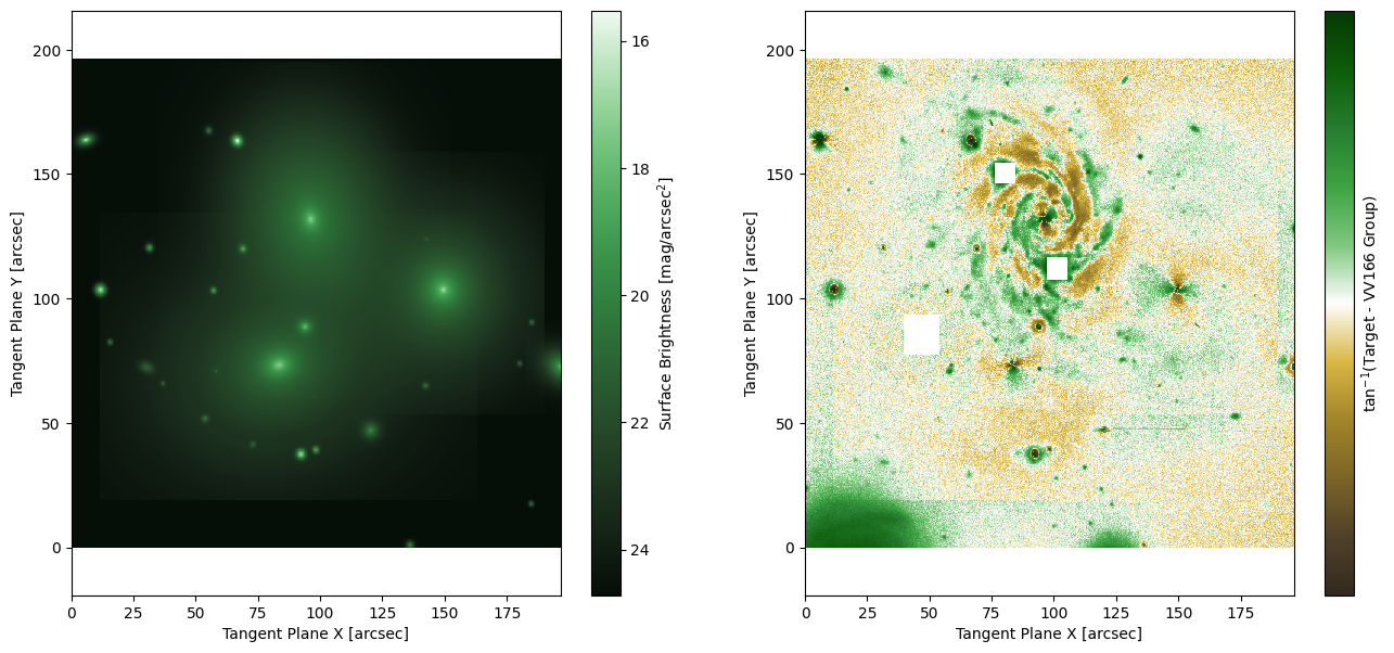
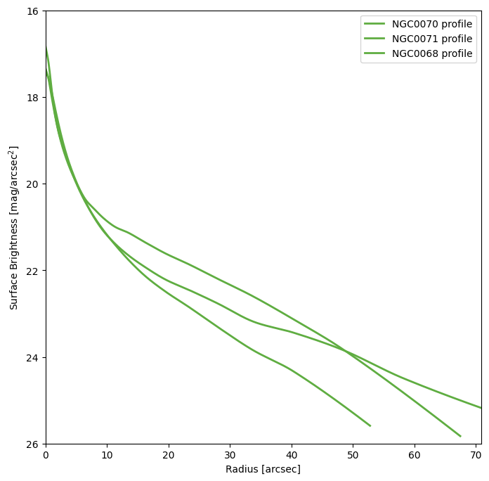
Now that’s starting to look like a complete model, and the Chi^2/ndf is much lower! And all for very little effort considering the level of detail. Looking at the residuals there is a clear improvement from the other attempts, that said there is a lot of structure in the residuals around the small objects, suggesting that a sersic alone is not the best model for these galaxies. That’s not too surprising, at the very least we should apply PSF convolution to the models to get the proper blurring. PSF convolution is very slow though, so it would be best to do on a GPU, which you can try out if you have access to one! Simply set psf_mode = “full” and run fit again. For now though, we’ll forgo the PSF convolution in the interest of time.

# and we can also take a look at the three main object profiles

fig8, ax8 = plt.subplots(figsize = (8,8))
# let's just plot the 3 main object profiles
for M in VV166Group.models.values():
    if not "NGC" in M.name: continue
    ap.plots.radial_light_profile(fig8, ax8, M)
ax8.legend()
ax8.set_ylim([26,16])
plt.show()